Mathematical Concepts and LaTeX Examples

This notebook demonstrates various mathematical concepts with LaTeX notation and visualizations using Python.

Topics Covered

Basic calculus concepts
Linear algebra
Probability and statistics
Fourier analysis

1. Calculus - Derivatives and Integrals

The derivative of a function $f(x)$ is defined as:

$$f’(x) = \lim_{h \to 0} \frac{f(x+h) - f(x)}{h}$$

For example, let’s consider the function $f(x) = x^2 \sin(x)$. Its derivative is:

$$f’(x) = 2x \sin(x) + x^2 \cos(x)$$

import numpy as np
import matplotlib.pyplot as plt
import seaborn as sns
from scipy import integrate

# Set up the plotting style
plt.style.use('seaborn-v0_8')
sns.set_palette("husl")

# Define the function and its derivative
def f(x):
    return x**2 * np.sin(x)

def f_prime(x):
    return 2*x*np.sin(x) + x**2*np.cos(x)

# Generate x values
x = np.linspace(-2*np.pi, 2*np.pi, 1000)

# Calculate function values
y = f(x)
y_prime = f_prime(x)

# Plot the function and its derivative
fig, (ax1, ax2) = plt.subplots(2, 1, figsize=(10, 8))

# Plot the function
ax1.plot(x, y, 'b-', linewidth=2, label='$f(x) = x^2 \sin(x)$')
ax1.set_title('Function $f(x) = x^2 \sin(x)$', fontsize=14)
ax1.set_ylabel('$f(x)$', fontsize=12)
ax1.grid(True, alpha=0.3)
ax1.legend()

# Plot the derivative
ax2.plot(x, y_prime, 'r-', linewidth=2, label="$f'(x) = 2x \sin(x) + x^2 \cos(x)$")
ax2.set_title('Derivative $f\'(x)$', fontsize=14)
ax2.set_xlabel('$x$', fontsize=12)
ax2.set_ylabel("$f'(x)$", fontsize=12)
ax2.grid(True, alpha=0.3)
ax2.legend()

plt.tight_layout()
plt.show()

<>:28: SyntaxWarning: invalid escape sequence '\s'
<>:29: SyntaxWarning: invalid escape sequence '\s'
<>:35: SyntaxWarning: invalid escape sequence '\s'
<>:28: SyntaxWarning: invalid escape sequence '\s'
<>:29: SyntaxWarning: invalid escape sequence '\s'
<>:35: SyntaxWarning: invalid escape sequence '\s'
/tmp/ipykernel_2802022/74342987.py:28: SyntaxWarning: invalid escape sequence '\s'
  ax1.plot(x, y, 'b-', linewidth=2, label='$f(x) = x^2 \sin(x)$')
/tmp/ipykernel_2802022/74342987.py:29: SyntaxWarning: invalid escape sequence '\s'
  ax1.set_title('Function $f(x) = x^2 \sin(x)$', fontsize=14)
/tmp/ipykernel_2802022/74342987.py:35: SyntaxWarning: invalid escape sequence '\s'
  ax2.plot(x, y_prime, 'r-', linewidth=2, label="$f'(x) = 2x \sin(x) + x^2 \cos(x)$")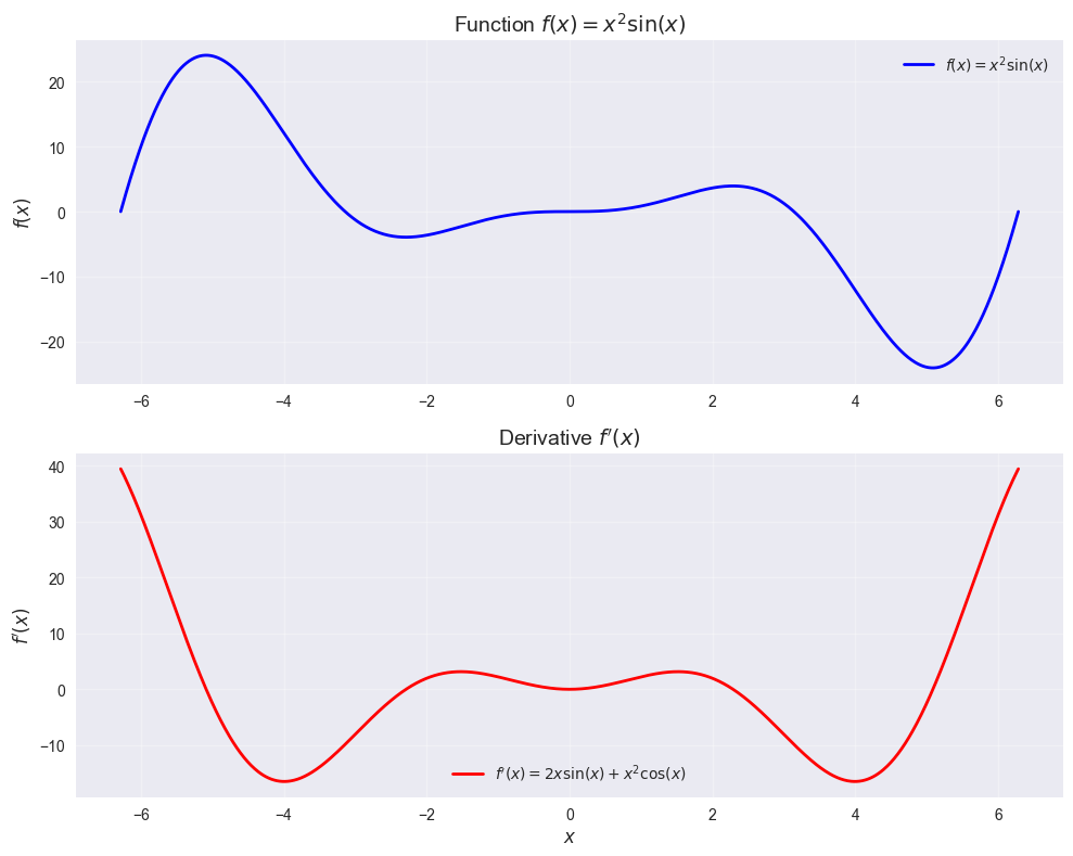

png

2. Linear Algebra - Eigenvalues and Eigenvectors

For a matrix $A$, an eigenvector $v$ and eigenvalue $\lambda$ satisfy:

$$Av = \lambda v$$

The characteristic polynomial is given by:

$$\det(A - \lambda I) = 0$$

# Create a sample matrix
A = np.array([[3, 1, 0],
              [1, 2, 1],
              [0, 1, 3]])

# Calculate eigenvalues and eigenvectors
eigenvalues, eigenvectors = np.linalg.eig(A)

print("Matrix A:")
print(A)
print("\nEigenvalues:")
for i, λ in enumerate(eigenvalues):
    print(f"λ_{i+1} = {λ:.4f}")

print("\nCorresponding eigenvectors:")
for i, v in enumerate(eigenvectors.T):
    print(f"v_{i+1} = {v}")

# Verify the eigenvalue equation Av = λv
print("\nVerification of Av = λv:")
for i, (λ, v) in enumerate(zip(eigenvalues, eigenvectors.T)):
    Av = A @ v
    λv = λ * v
    print(f"Eigenpair {i+1}: ||Av - λv|| = {np.linalg.norm(Av - λv):.2e}")

Matrix A:
[[3 1 0]
 [1 2 1]
 [0 1 3]]

Eigenvalues:
λ_1 = 1.0000
λ_2 = 3.0000
λ_3 = 4.0000

Corresponding eigenvectors:
v_1 = [ 0.40824829 -0.81649658  0.40824829]
v_2 = [ 7.07106781e-01  4.02240178e-16 -7.07106781e-01]
v_3 = [0.57735027 0.57735027 0.57735027]

Verification of Av = λv:
Eigenpair 1: ||Av - λv|| = 4.78e-16
Eigenpair 2: ||Av - λv|| = 2.62e-15
Eigenpair 3: ||Av - λv|| = 1.83e-15

# Visualize the eigenvectors
fig, ax = plt.subplots(1, 1, figsize=(8, 6))

# Plot the eigenvectors
colors = ['red', 'blue', 'green']
for i, (λ, v) in enumerate(zip(eigenvalues, eigenvectors.T)):
    ax.arrow(0, 0, v[0], v[1], head_width=0.1, head_length=0.1, 
            fc=colors[i], ec=colors[i], linewidth=2,
            label=f'$v_{i+1}$ (λ_{i+1} = {λ:.2f})')

ax.set_xlim(-1, 1)
ax.set_ylim(-1, 1)
ax.set_aspect('equal')
ax.grid(True, alpha=0.3)
ax.set_title('Eigenvectors of Matrix A', fontsize=14)
ax.set_xlabel('$x_1$', fontsize=12)
ax.set_ylabel('$x_2$', fontsize=12)
ax.legend()
plt.show()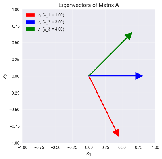

png

3. Probability and Statistics

Normal Distribution

The probability density function of a normal distribution is:

$$f(x) = \frac{1}{\sigma\sqrt{2\pi}} e^{-\frac{1}{2}\left(\frac{x-\mu}{\sigma}\right)^2}$$

where $\mu$ is the mean and $\sigma$ is the standard deviation.

from scipy import stats

# Define parameters for normal distribution
μ = 0  # mean
σ = 1  # standard deviation

# Create normal distribution
norm_dist = stats.norm(μ, σ)

# Generate x values
x = np.linspace(-4, 4, 1000)

# Calculate PDF and CDF
pdf = norm_dist.pdf(x)
cdf = norm_dist.cdf(x)

# Plot PDF and CDF
fig, (ax1, ax2) = plt.subplots(1, 2, figsize=(12, 5))

# Plot PDF
ax1.plot(x, pdf, 'b-', linewidth=2, label=f'N({μ}, {σ}²)')
ax1.fill_between(x, pdf, alpha=0.3)
ax1.set_title('Probability Density Function', fontsize=14)
ax1.set_xlabel('$x$', fontsize=12)
ax1.set_ylabel('$f(x)$', fontsize=12)
ax1.grid(True, alpha=0.3)
ax1.legend()

# Plot CDF
ax2.plot(x, cdf, 'r-', linewidth=2, label=f'N({μ}, {σ}²)')
ax2.set_title('Cumulative Distribution Function', fontsize=14)
ax2.set_xlabel('$x$', fontsize=12)
ax2.set_ylabel('$F(x)$', fontsize=12)
ax2.grid(True, alpha=0.3)
ax2.legend()

plt.tight_layout()
plt.show()

# Calculate some statistics
print(f"Mean: {norm_dist.mean():.4f}")
print(f"Variance: {norm_dist.var():.4f}")
print(f"Standard deviation: {norm_dist.std():.4f}")
print(f"Skewness: {norm_dist.stats('s'):.4f}")
print(f"Kurtosis: {norm_dist.stats('k'):.4f}")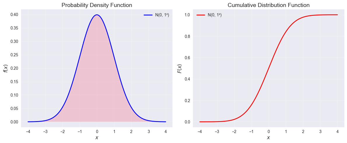

png

Mean: 0.0000
Variance: 1.0000
Standard deviation: 1.0000
Skewness: 0.0000
Kurtosis: 0.0000

Central Limit Theorem

The Central Limit Theorem states that the sum of $n$ independent and identically distributed random variables approaches a normal distribution as $n \to \infty$.

Mathematically: $\frac{\bar{X}_n - \mu}{\sigma/\sqrt{n}} \xrightarrow{d} N(0, 1)$

# Demonstrate Central Limit Theorem
def demonstrate_clt(sample_size, n_experiments, distribution='uniform'):
    """
    Demonstrate the Central Limit Theorem
    """
    sample_means = []
    
    for _ in range(n_experiments):
        if distribution == 'uniform':
            # Uniform distribution U(0, 1)
            samples = np.random.uniform(0, 1, sample_size)
        elif distribution == 'exponential':
            # Exponential distribution with λ = 1
            samples = np.random.exponential(1, sample_size)
        
        sample_means.append(np.mean(samples))
    
    return np.array(sample_means)

# Parameters
sample_sizes = [1, 5, 10, 30, 50]
n_experiments = 1000

# Generate sample means for different sample sizes
fig, axes = plt.subplots(2, 3, figsize=(15, 10))
axes = axes.flatten()

for i, n in enumerate(sample_sizes):
    sample_means = demonstrate_clt(n, n_experiments, 'uniform')
    
    # Plot histogram
    axes[i].hist(sample_means, bins=30, density=True, alpha=0.7, 
                color='skyblue', edgecolor='black')
    
    # Overlay normal distribution
    x = np.linspace(sample_means.min(), sample_means.max(), 100)
    theoretical_mean = 0.5  # Mean of U(0,1)
    theoretical_std = np.sqrt(1/12) / np.sqrt(n)  # Std of U(0,1) / sqrt(n)
    normal_pdf = stats.norm.pdf(x, theoretical_mean, theoretical_std)
    axes[i].plot(x, normal_pdf, 'r-', linewidth=2, label='Normal approximation')
    
    axes[i].set_title(f'n = {n}', fontsize=12)
    axes[i].set_xlabel('Sample Mean', fontsize=10)
    axes[i].set_ylabel('Density', fontsize=10)
    axes[i].legend()
    axes[i].grid(True, alpha=0.3)

# Remove the last subplot (empty)
axes[-1].axis('off')

plt.suptitle('Central Limit Theorem Demonstration', fontsize=16)
plt.tight_layout()
plt.show()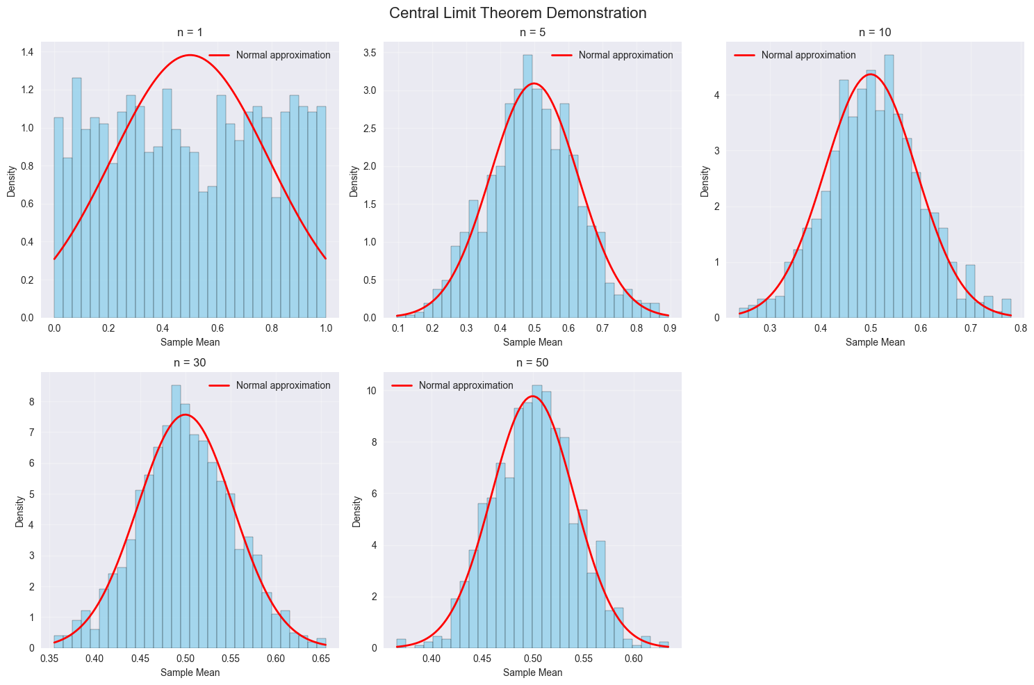

png

4. Fourier Analysis

The Fourier transform of a function $f(t)$ is defined as:

$$F(\omega) = \int_{-\infty}^{\infty} f(t) e^{-i\omega t} dt$$

The inverse Fourier transform is:

$$f(t) = \frac{1}{2\pi} \int_{-\infty}^{\infty} F(\omega) e^{i\omega t} d\omega$$

# Generate a composite signal
t = np.linspace(0, 2, 1000)  # Time vector

# Create a signal with multiple frequency components
signal = (np.sin(2 * np.pi * 1 * t) +           # 1 Hz component
          0.5 * np.sin(2 * np.pi * 3 * t) +     # 3 Hz component
          0.3 * np.sin(2 * np.pi * 5 * t) +     # 5 Hz component
          0.1 * np.random.normal(0, 1, len(t))) # Noise

# Compute FFT
fft_result = np.fft.fft(signal)
frequencies = np.fft.fftfreq(len(t), t[1] - t[0])

# Only keep positive frequencies
positive_freq_idx = frequencies > 0
frequencies = frequencies[positive_freq_idx]
fft_magnitude = np.abs(fft_result[positive_freq_idx])

# Plot the signal and its frequency spectrum
fig, (ax1, ax2) = plt.subplots(2, 1, figsize=(12, 8))

# Plot time domain signal
ax1.plot(t, signal, 'b-', linewidth=1)
ax1.set_title('Time Domain Signal', fontsize=14)
ax1.set_xlabel('Time (s)', fontsize=12)
ax1.set_ylabel('Amplitude', fontsize=12)
ax1.grid(True, alpha=0.3)

# Plot frequency spectrum
ax2.plot(frequencies[:50], fft_magnitude[:50], 'r-', linewidth=2)
ax2.set_title('Frequency Spectrum (FFT)', fontsize=14)
ax2.set_xlabel('Frequency (Hz)', fontsize=12)
ax2.set_ylabel('Magnitude', fontsize=12)
ax2.grid(True, alpha=0.3)
ax2.set_xlim(0, 10)

# Mark the known frequency components
for freq, amplitude in [(1, 2), (3, 1), (5, 0.6)]:
    ax2.axvline(x=freq, color='green', linestyle='--', alpha=0.7)
    ax2.text(freq, amplitude, f'{freq} Hz', rotation=90, 
             verticalalignment='bottom', fontsize=10)

plt.tight_layout()
plt.show()

# Identify peak frequencies
from scipy.signal import find_peaks
peaks, _ = find_peaks(fft_magnitude[:50], height=0.1)
peak_frequencies = frequencies[peaks]
peak_magnitudes = fft_magnitude[peaks]

print("Detected frequency components:")
for freq, mag in zip(peak_frequencies, peak_magnitudes):
    print(f"Frequency: {freq:.2f} Hz, Magnitude: {mag:.2f}")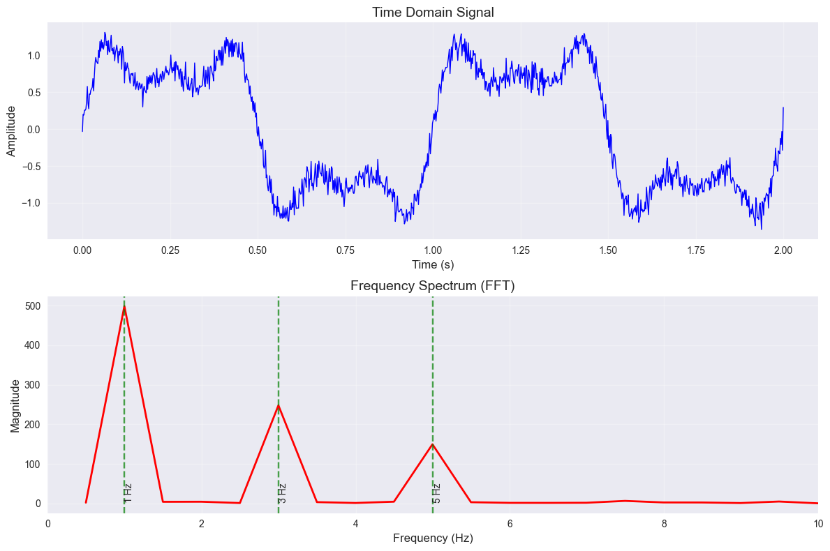

png

Detected frequency components:
Frequency: 1.00 Hz, Magnitude: 498.73
Frequency: 2.00 Hz, Magnitude: 4.35
Frequency: 3.00 Hz, Magnitude: 247.95
Frequency: 4.99 Hz, Magnitude: 149.55
Frequency: 7.49 Hz, Magnitude: 6.45
Frequency: 9.49 Hz, Magnitude: 4.86
Frequency: 11.99 Hz, Magnitude: 3.51
Frequency: 13.49 Hz, Magnitude: 5.52
Frequency: 14.49 Hz, Magnitude: 4.49
Frequency: 15.98 Hz, Magnitude: 4.24
Frequency: 16.98 Hz, Magnitude: 2.52
Frequency: 17.98 Hz, Magnitude: 3.71
Frequency: 19.48 Hz, Magnitude: 4.62
Frequency: 20.48 Hz, Magnitude: 4.22
Frequency: 22.48 Hz, Magnitude: 4.40
Frequency: 23.98 Hz, Magnitude: 3.12

Summary

This notebook demonstrated several important mathematical concepts:

Calculus: Derivatives and their visualization
Linear Algebra: Eigenvalues and eigenvectors
Probability: Normal distribution and Central Limit Theorem
Fourier Analysis: Signal decomposition in frequency domain

Each section included mathematical notation using LaTeX and corresponding Python implementations for visualization and computation.

Mathematical Concepts and LaTeX Examples

Mathematical Concepts and LaTeX Examples

Topics Covered

1. Calculus - Derivatives and Integrals

2. Linear Algebra - Eigenvalues and Eigenvectors

3. Probability and Statistics

Normal Distribution

Central Limit Theorem

4. Fourier Analysis

Summary

Keyboard Shortcuts

Vim Navigation

Utilities

Left Bar

Right Bar

Appearance